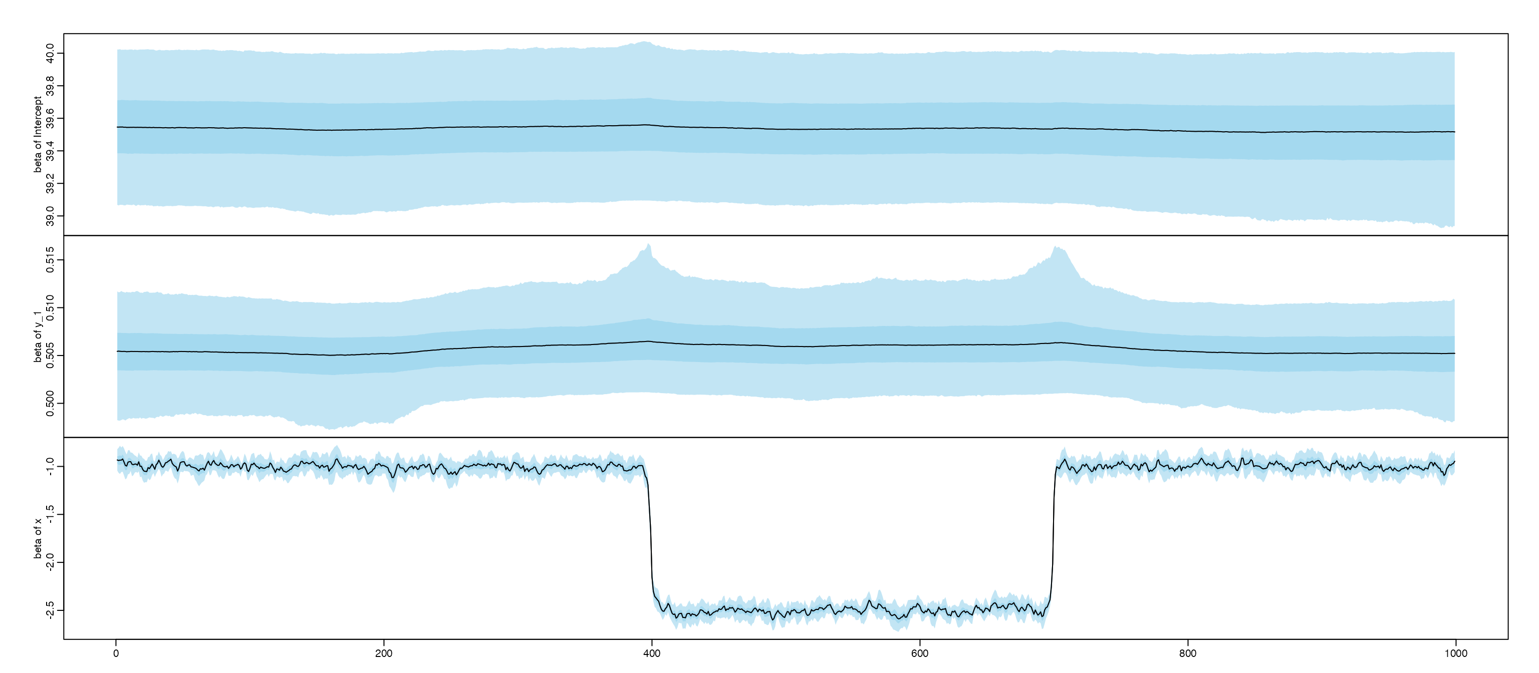
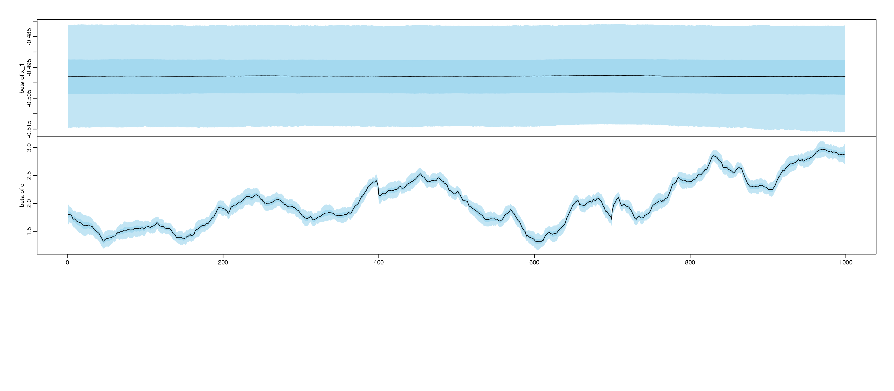
As we mentioned in the Quick start, we usually need an initial guess
of formula, and set up the ss_param and
cpt_learning_param, this requires our knowledge of each
coefficient \(\beta_{j,t}\) and we will
ask questions of whether this variables should goes into our model, what
is the state-space equation, what is an appropriate initial value and if
there is any change point. Sometimes this question can be answered by
domain knowledge. Here we provide a function for an automatically
exploration and help users identify the formula and parameters as easy
as a one line code. The idea is based on shrinkTVP which
incorporates Bayesian hierarchical shrinkage for state-space model, to
achieve a two-way sparsity. Details can be found:..
head(data_complex)
#>         Date        y          x         c      y_1        x_1
#> 2 2020-02-07 79.43535 12.3290419  6.145098 82.18145  2.4949289
#> 3 2020-02-08 75.06166  5.2927101  3.655687 79.43535 12.3290419
#> 4 2020-02-09 85.71720  0.9862238  6.413653 75.06166  5.2927101
#> 5 2020-02-10 83.22922  7.6992702  4.533435 85.71720  0.9862238
#> 6 2020-02-11 88.17003 11.7192263 11.722012 83.22922  7.6992702
#> 7 2020-02-12 86.50519 10.2398440 10.196931 88.17003 11.7192263
res = shrinkTVP(formula = y ~ y_1 + x + x_1 + c, data = data_complex)
We start our exploration:
SSMimpute::explore_SSM(res = res)
#> Hit <Return> to see next plot:

#> Warning: `as.tibble()` was deprecated in tibble 2.0.0.
#> ℹ Please use `as_tibble()` instead.
#> ℹ The signature and semantics have changed, see `?as_tibble`.
#> ℹ The deprecated feature was likely used in the SSMimpute package.
#>   Please report the issue at
#>   <
#> # A tibble: 5 × 7
#>   coef        mean      sd median   HPD1   HPD2 ESS.var1
#>   <chr>      <dbl>   <dbl>  <dbl>  <dbl>  <dbl>    <dbl>
#> 1 Intercept 39.5   0.244   39.5   39.1   40.0        549
#> 2 y_1        0.505 0.00337  0.505  0.498  0.512      217
#> 3 x         -0.929 0.102   -0.928 -1.13  -0.729      936
#> 4 x_1       -0.498 0.00853 -0.498 -0.515 -0.482     1038
#> 5 c          1.80  0.112    1.80   1.57   2.01       392
#> Press [enter] to see the non-stationary coefficient:
#> # A tibble: 2 × 7
#>   variance   mean      sd median   HPD1   HPD2 ESS.var1
#>   <chr>     <dbl>   <dbl>  <dbl>  <dbl>  <dbl>    <dbl>
#> 1 x        0.0577 0.00258 0.0577 0.0524 0.0625      733
#> 2 c        0.0422 0.00310 0.0421 0.0361 0.0483      263
#> indicating non-stationary process for:  x c ;
#> Press [enter] to further checking for change points:

#> Press [enter] to further checking fitted ARIMA model
#> Series: B_1
#> ARIMA(1,1,0)
#>
#> Coefficients:
#>          ar1
#>       0.4839
#> s.e.  0.0277
#>
#> sigma^2 = 0.001111:  log likelihood = 1980.47
#> AIC=-3956.94   AICc=-3956.93   BIC=-3947.13
#>
#> Training set error measures:
#>                        ME       RMSE        MAE          MPE     MAPE     MASE
#> Training set 2.193772e-06 0.03330578 0.01969118 -0.003620092 1.573118 1.014929
#>                     ACF1
#> Training set -0.01128863
#> Series: B_1
#> ARIMA(2,1,1)
#>
#> Coefficients:
#>          ar1      ar2      ma1
#>       1.0653  -0.1848  -0.5873
#> s.e.  0.1188   0.0820   0.1102
#>
#> sigma^2 = 0.0002044:  log likelihood = 2827.31
#> AIC=-5646.63   AICc=-5646.58   BIC=-5627
#>
#> Training set error measures:
#>                        ME       RMSE         MAE        MPE      MAPE      MASE
#> Training set 0.0003202908 0.01426679 0.009208638 0.01774389 0.4719043 0.7113199
#>                      ACF1
#> Training set -0.002916669
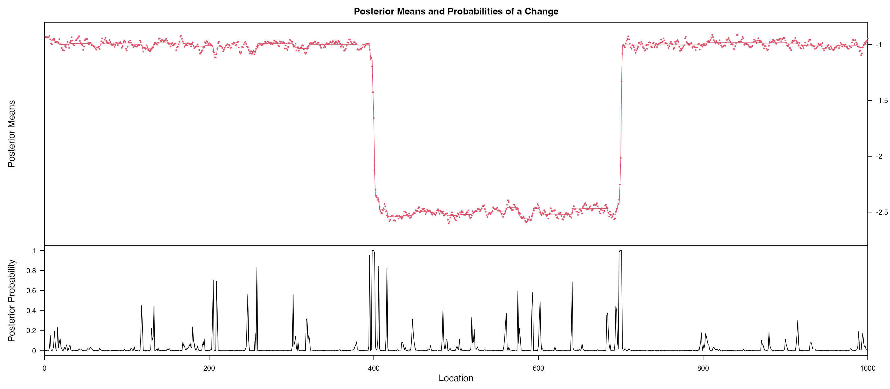
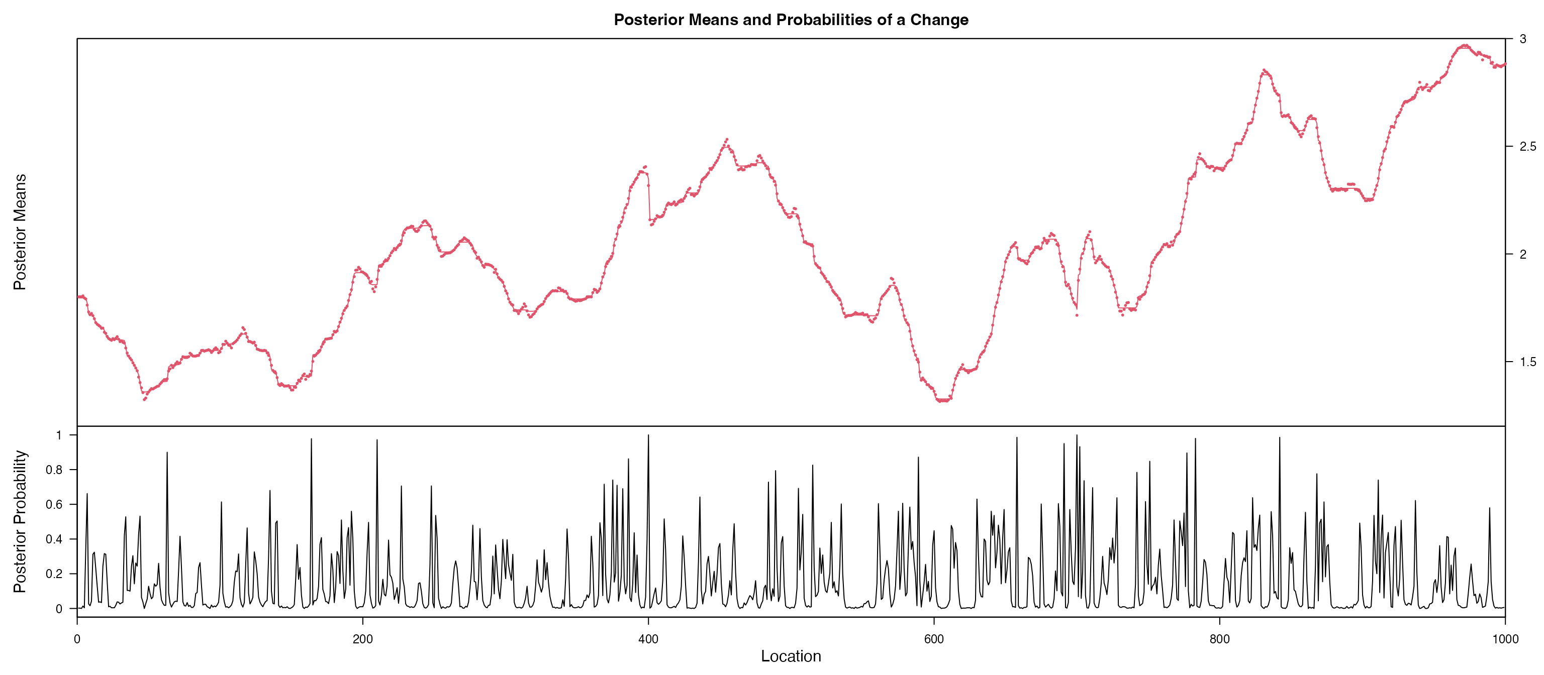
Based on the figures, we notice coefficient of x and
c are probably non-stationary, we further using
bcp for a Bayesian change point detection, gives a
posterior probability of change point in each change point. We notice a
clear change point for x is 400 and 700. and the coefficent
for c is probably a random walk.